A New View of Statistics	© 2000 Will G Hopkins
Go to: Next · Previous · Contents · Search · Home

Generalizing to a Population: CONFIDENCE LIMITS continued

From the point of view of confidence intervals, getting it wrong is simply a matter of the population value being outside the confidence interval. I call it a Type O error. You can think of the "O" as standing either for "outside (the confidence interval)" or for "zero" (as opposed to errors of Type I and II, which it supersedes). For 95% confidence limits the Type O error rate is 5%, by definition. From the point of view of hypothesis testing, getting it wrong is much more complicated. You can be responsible for a false alarm or Type I error, and a failed alarm or Type II error. An entirely different way to get things wrong is to have bias in your estimate of an effect. This page ends with a link to download a PowerPoint slide presentation, in which I summarize and in some instances extend important points from these pages.

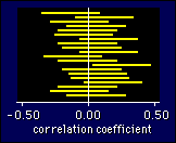
For example, here are typical 95% confidence intervals for 20 samples of the same size for a population in which the correlation is 0.00. (The sample size is irrelevant.) Notice that one of the correlations is statistically significant. If that happened to be your study, you would rush into print saying that there is a correlation, when in reality there isn't. You would be the victim of a Type I error. Of course, you wouldn't know until others--or you--had tested more subjects and found a narrower confidence interval overlapping zero.

Cumulative Type I and Type O Error Rates
The only time you need to worry about setting the Type I error rate is when you look for a lot of effects in your data. The more effects you look for, the more likely it is that you will turn up an effect that seems bigger than it really is. This phenomenon is usually called the inflation of the overall Type I error rate, or the cumulative Type I error rate. So if you're going fishing for relationships amongst a lot of variables, and you want your readers to believe every "catch" (significant effect), you're supposed to reduce the Type I error rate by adjusting the p value downwards for declaring statistical significance.

The simplest adjustment is called the Bonferroni. For example, if you do three tests, you should reduce the p value to 0.05/3, or about 0.02. This adjustment follows quite simply from the meaning of probability, on the assumption that the three tests are independent. If the tests are not independent, the adjustment is too severe.

Those of us who use confidence intervals rather than p values have to be aware that inflation of the Type O error also happens when we report more than one effect. For example, if there are two independent effects, the probability that at least one will be outside its confidence interval is about 10%. We could increase the width of our confidence intervals to bring the overall probability back to 5%. For example, Bonferroni-adjusted 95% confidence intervals for three effects would each be 98% confidence intervals. Adjusting the confidence intervals in this or some other way will keep the purists happy, but I'm not sure it's such a good idea. I prefer to see the raw 95% confidence intervals, and I prefer to make my own mental adjustment when there are lots of effects. I just look at the results and think to myself, OK, the population value might be outside the interval for one or two of those effects (depending on how many results are reported). The fact that the effects are reported in one publication is no justification for widening the confidence intervals, in my view. You might just as well argue that all the confidence intervals in the entire issue of the journal should be widened, to keep the cumulative error rate for the issue in check! And why stop with one issue... So I don't think confidence intervals or p values should be adjusted, but I know many will disagree.

Why not use a lower p value all the time, for example a p value of 0.01, to declare significance? Surely that way only one in every 100 effects you test for is likely to be bogus? Yes, but it is harder to get significant results, unless you use a bigger sample to narrow down that confidence interval. In any case, you are entitled to stay with a 5% level for one or two tests, if they are pre-planned--in other words, if you set up the whole study just to do these tests. It's only when you tack on a lot of other tests afterwards (so-called post-hoc tests) that you need to be wary of false alarms.

Controlling the Type I error comes up a lot in analysis of variance, when you do comparisons between several groups or levels. For more insights see estimates and contrasts in one-way ANOVA and estimates and contrasts in repeated-measures ANOVA.

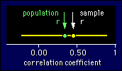
The smaller the sample, the more likely you are to commit a Type II error, because the confidence interval is wider and is therefore more likely to overlap zero. Here's an example in which a Type II error has occurred for a correlation. Imagine you got this result:

I've indicated where the population correlation is for this example, but of course, in reality you wouldn't know where it was. I've made the true correlation about 0.40, which is well worth detecting. But it hasn't been detected, because the confidence interval overlaps zero. A big-enough sample size would have produced a confidence interval that didn't overlap zero, in which case you would have detected a correlation, so no Type II error would have occur red. Now, a test of your understanding: where would the population r have to be on the figure for a Type II error NOT to have been made? Answer: on or close to 0.00.

The Type II error needs to be considered explicitly at the time you design your study. That's when you're supposed to work out the sample size needed to make sure your study has the power to detect anything useful. For this purpose the usual Type II error rate is set to 20%, or 10% for really classy studies. The power of the study is sometimes referred to as 80% (or 90% for a Type II error rate of 10%). In other words, the study has enough power to detect the smallest worthwhile effects 80% (or 90%) of the time.

Here's something interesting that no-one seems to mention: cumulative Type II error rate--in other words, the chance that you will miss at least one effect when you test for more than one. Is your head starting to spin? Mine is! Don't worry, just go back to confidence limits and the notion of cumulative Type O error. When you are looking at lots of effects, the near equivalent of inflated Type II error is the increased chance that any one of the effects will be bigger than you think it could be (bigger than its upper confidence limit). Come to think of it, the near equivalent of inflated Type I error is the increased chance that any one of the effects will be smaller than you think.

The easiest way to get bias is to use a sample that is in some way a non-random sample of the population: if the average subject in the sample tends to be different from the average person in the population, the effect you are looking at could well be different in the sample compared with the population.

Some statistics are biased, if we calculate them in the wrong way. Using n instead of n-1 to work out a standard deviation is a good example. There is also bias in some reliability statistics. Building up a sample size in stages can also result in bias, as I describe in sample size on the fly.