A New View of Statistics	© 2003 Will G Hopkins
Go to: Next · Previous · Contents · Search · Home

Generalizing to a Population:
REPEATED-MEASURES MODELS continued

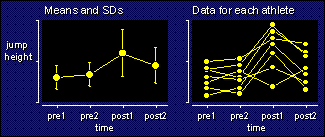
Check back and you'll see it's the same model as for two trials with no between-subjects effect: adding extra trials doesn't usually mean a different model. This kind of design--multiple repeated measurements without a control group--is sometimes called a time series. In the above example, there are two trials (pre1 and pre2) to establish a baseline of performance before some kind of treatment, then two trials (post1 and post2) to see the effect of the treatment. There's a big effect at post1, but it's wearing off by post2.

One way to analyze these data is to do a series of paired t tests. Post1 vs pre2 is the first comparison you would want to do. You'd also be interested in post2 vs post1, and possibly pre2 vs pre1, post 1 vs the mean of pre1 and pre2, and so on. An analysis that takes into account all the tests is more elegant and more powerful. The trouble is, generally we can't analyze such data using conventional ANOVA. The example shows several reasons why. See if you can spot them before reading on.

You should have noticed that the standard deviation is bigger for the post1 and post2 trials. Different SDs are a problem for conventional ANOVA, but if that was the only problem, we could fix it by doing a non-parametric analysis via rank transformation of the dependent variable. No, the real problems are apparent only when you look at the data for the individual athletes. One of them appears to be a negative responder to the training program, and another is possibly a non-responder. What's more, the ordering of the subjects between pre2 and post1 or between post1 and post2 was not nearly as good as the ordering between the baseline tests. It's this change in consistency of ordering, or to give it its statistical term, the change in reliability between tests, that stymies the normal ANOVA. Individual differences in the response to the treatment between subjects is the reason for the loss of ordering here.

A change in reliability shows up as different correlations between pre1 and pre2, pre2 and post1, etc. When these correlations get too different and/or the standard deviations get too different, it's called loss of sphericity or asphericity. Statisticians examine sphericity in something called a covariance matrix, which neatly summarizes correlations and standard deviations for all the levels of the within-subject effect (time or trial). I will provide more information about covariances soon on the page devoted to the use of Proc Mixed in the Statistical Analysis System. Meanwhile, let's look at the three fixes for this problem.
 
Fix #1: Multivariate ANOVA
 Someone worked out that you can treat the values of the dependent variable for each trial as separate dependent variables. In our example, jumphgt becomes jumphgt1 (values at pre1), jumphgt2 (values at pre2), etc. The data set would look like this:

jumphgt1	jumphgt2	jumphgt3	jumphgt4
163	165	171	168
167	166	170	167
etc.	etc.	etc.	etc.

Notice that time as a variable has disappeared: it's been absorbed into the four new variables for jump height, but it reappears as a within-subjects factor when you run the analysis. The variable subject has also disappeared: it's not needed, because there is only one row per subject and no ambiguity is possible.

It's difficult to write these four new variables into a model. Obviously they go on the left-hand side, like so:

jumphgt1  jumphgt2  jumphgt3  jumphgt4 <=

but what goes on the right-hand side? Nothing! Looks silly, but SAS makes you show it like this when you analyze a data set like the above.

I don't recommend the multivariate ANOVA approach. For starters, all it provides is a p value for the overall effect of time. It doesn't provide estimates or p values for the individual contrasts of interest (post1 minus pre2 etc.). What's more, I've shown by doing simulations that the p value it does produce is too big with some kinds of data and too small with others. Another big problem is missing values: if one of your subjects missed one of the tests, that subject is omitted from the analysis entirely.
 
Fix #2: Adjusted Univariate ANOVA
 This method has been the most widely used. The analysis is done as a conventional two-way ANOVA with one dependent variable (hence univariate) and effects for subject and trial (time in our example). The program then uses the covariance matrix to come up with a correction factor that leads to a different p value for the effect of trial. You choose from two factors: Greenhouse-Geisser epsilon or Huynh-Feldt epsilon.
 
Fix #3: Within-subject Modeling
 In this approach, you avoid the problems of repeated measures by not doing them! Instead, you convert each subject's repeated measurements into a single number, then do paired or unpaired t tests or simple ANOVAs on those numbers. I explain this approach later and in the slideshow.
 
Fix #4: Modeling Covariances (Mixed Models)
 Suppose you have data like the previous example, where the standard deviations and correlations for the repeated measures are all over the place. Don't adjust for them: make them part of the model! Yes you can, with Proc Mixed in the Statistical Analysis System (SAS). It's a major breakthrough. The procedure is known as modeling covariances, because standard deviations and correlations can be expressed more generally as covariances (nothing to do with analysis of covariance, by the way). Unfortunately the instructions for the procedure that does it in SAS are incomprehensible to all but highly trained statisticians. But if you can find one of those, you will be delighted, for the following reasons:

• This method of modeling can handle missing values! No longer do you lose the entire data for a subject who missed one or two tests.
• You can dial up just about any structure of standard deviations and correlations.
• The model starts to look like a proper univariate ANOVA again. Unfortunately you still don't specify the subject term in a natural way (as an overt effect in the model), not in SAS anyway. The model statement is reserved for fixed effects. The model for our example would be jumphgt <= time. You specify the identity of subjects as a random effect.
• The data set is submitted in the more natural univariate format. For example:

  athlete	time	jumphgt
  Jo	pre1	163
  Jo	pre2	165
  Jo	post1	171
  Jo	post2	168
  Kim	pre1	167
  etc.	etc.	etc.

By the way, the term mixed refers either to the fact that you are modeling a mixture of means and covariances, or (same thing) to the fact the model consists of a mixture of random and fixed effects. The subject term in a repeated-measures model is a random effect. Random effects produce variance that has to be accounted for in the model.

I have now added SAS programs for analyzing repeated-measures data with the mixed procedure in SAS. Link to them from the page devoted to Proc Mixed.
 
Estimates or Contrasts
 OK, let's assume we've got a method that accounts for lack of sphericity. Now for the question of estimates or contrasts between the mean jump heights at the different times. You can dial up any contrast you like, if you and the stats program are good enough! For example, was the jump height straight after the intervention higher than the mean of the baseline values (and what's the confidence interval on the difference)? Some stats programs offer standard contrasts. Examples: One level with every other, would be the obvious contrast to apply to post1 in the above example. Each level with the one immediately preceding is good for determining where a change takes place in a time course, although you can easily get the situation where no successive contrasts are significant, and yet there is obviously a significant trend upwards or downwards. That's where polynomial contrasts come to the rescue: the ANOVA procedure fits a straight line, and/or a quadratic, and/or a cubic, etc. to the means.

Polynomial Contrasts
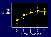
 Here's an example of data that would be ideally suited to fitting a straight line and a quadratic. It's jump height and time again, but I've added an extra time point and made a curvilinear trend:

The magnitude and significance of the linear component would tell you about the general upward trend in performance, while the quadratic component would tell you how it is leveling off with time. If your stats program's a good one, it will offer polynomial contrasts as an option. Otherwise you will need a high-powered helper to combine the levels of the time effect in a way that generates the coefficients of the polynomials. You can adjust for unequal intervals between the time points, too, if your stats program or helper are really good. (SAS users can fit a polynomial directly in the model with Proc Mixed.)

By the way, what if the data in the above figure were not repeated measures? In other words, what if there were different subjects at each time point? For example, the data could represent level of physical activity in samples drawn from a population at monthly intervals. Could you still do polynomial contrasts? Of course. You do it within a normal ANOVA.

Controlling Type I Error with Repeated Measures
 Keeping the overall chance of a type I error in check efficiently for multiple contrasts between levels of a repeated-measures factor seems to be theoretically difficult. The SAS program simply doesn't offer the option. I don't worry about it anyway, because I don't believe in testing hypotheses. If you are a p-value traditionalist, use the Bonferroni correction. And as I explained earlier, do specific estimates/contrasts regardless of the p value for the overall effect.