![]()
Repeated-Measures ANOVA with two trials plus a between-subjects effect
|
A New View of Statistics | |
|
|
Repeated-Measures ANOVA with two trials plus a between-subjects effect |
 Let's take the experiment on the previous
page, where we attempted to increase jump height with some sort of experimental
treatment. As before, we measure jump height pre and post the treatment in a group
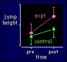
of subjects, the experimental group (expt in the figure). But now we also
have a second group who get a different treatment, and the aim of the experiment
is to compare the change in jump height in the two groups. If that different treatment
is nothing at all, or a sham treatment (a placebo), the second group is
called a control group--hence the name for this sort of experiment, a controlled
trial.
Let's analyze it the easy way first. For each subject, subtract the pre height from the post height to get a change score. Now compare the change scores in the two groups using an unpaired t test. Use the unequal-variances version of the t test, because the standard deviation (square root of the variance) of the change scores in the experimental group is likely to be larger than that in the control group, owing to individual responses to the treatment. The spreadsheet for controlled trials can do it all for you. If you have three groups (e.g. two experimental groups and one control group), use a new spreadsheet for each pairwise comparison of groups. You can also use a one-way ANOVA on the change scores, but beware: ANOVA assumes equal variances (standard deviations) of the change scores in all the groups. See the slide show on repeated measures for an explanation of these subtleties.
Now for the model, which is the hard way. We have to do it, though, because you need to understand the model for later complexities with repeated measures. Let's start with the simple model from the previous page:
jumphgt <= (athlete) time
This model represents the obvious fact that jump height is affected by time (depends whether it's the pre-test of the post-test) and the identity of the athlete (depends how good a jumper s/he is). But we now have two groups of subjects (control and expt), so we have to add a term to show that athletes in one group could jump differently from those in the other:
jumphgt <= (athlete) time group
Technically the model is now a three-way ANOVA, but no-one ever calls it that. OK, what tells us whether the experimental group did better in the post test, relative to the control group? The group effect? No, this term represents the overall difference between the groups, counting pre and post tests. We're missing a term, of course: the interaction time*group. This term is the first thing you look at to see how your treatment worked.. So the full model is:
jumphgt <= (athlete) time group time*group
By the way, the order of time and group in the model is irrelevant, and time*group is the same as group*time.
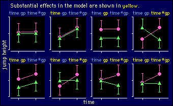
The data for this model seem simple enough (pre and post means and SDs for two groups), but interpreting the substantiveness/significance of each term in the model can be confusing. So here are examples illustrating the eight possible combinations of insubstantial and substantial effects for the different terms in the model. Don't go past this section until you understand all eight parts of this diagram:

The last two examples on the lower right are the ones we usually want in a study: no difference between the control and experimental groups in the pretest, and a nice big divergence on post-test. The fact that main effects are substantial in these two examples is irrelevant. The other two examples with a substantial interaction also illustrate treatments that worked, but the outcomes are not ideal, because in both cases the groups are different in the pretest. A worry, because it means that one or both of the groups can't be representative of the population, at least as far as jump height is concerned. And non-representative samples mean non-generalizable findings!
Finally how do we calculate the magnitude of the experimental effect? Easy.
The post score minus the pre score for the experimental group is the main thing,
but we have to subtract off any change in the control group. To do it as an
estimate or contrast in the repeated-measures ANOVA, combine the four levels
of time*group in the following way: (post·expt - pre·expt) - (post·cont
- pre·cont).
Special Case: Simple Crossovers
In a simple crossover
design, half the subjects get a control treatment followed by an experimental
treatment, while the other half get the treatments the other way around. People
usually analyze the data as a simple paired
t test, which means they effectively subtract the control response from
the experimental response for each subject, without regard for the order of
treatment. In a minute I'll show you a better way, using the above ANOVA model,
and I'll generalize it to multiple crossovers. First, more about simple crossovers.
Why split the subjects into two groups and cross the treatments over? Because if all subjects get the control and experimental treatments in the same order, you won't know whether any change you see is truly an effect of the treatment, or just an effect of being tested a second time--a practice or learning effect. When you split the subjects, the group that gets the control first has the practice effect added to the experimental treatment, whereas the group that gets the experimental first has the practice effect added to the control treatment. So when you average the difference scores, the practice effect disappears and you are left with the treatment effect, provided the two groups have the same number of subjects.
Fine, but there's a problem. When there is a practice effect, you get two clusters of difference scores. For example, if the practice effect is about the same size as the treatment effect, one set of difference scores will be around zero, and the other will tend to be twice as large as the treatment effect. The average is still equal to the treatment effect, but the effect appears to be more variable between subjects. The result is a bigger (worse) confidence interval for the treatment effect, or a bigger (worse) p value, or less power to detect the treatment effect.
Another potential problem is carry over. For the group that gets the experimental treatment first, it's important that any effect of the treatment disappears by the time that group gets the control treatment--otherwise the difference between control and experimental treatments for that group will be reduced. The result will be an apparently smaller treatment effect overall, and an apparent practice effect. For example, if the treatment effect carries over completely, the analysis will produce a treatment effect that is half its true value, and an apparent practice effect of the same magnitude. So you can't do a training study as a crossover, unless you are confident that the adaptations produced by the experimental training program decay away before subjects get the control program.
You might be able to get over the problem of carry over by increasing the time between the two treatments. But the longer the time, the less reliable the dependent variable is likely to be, which means a wider confidence interval for the difference between the treatments.
One way around the problem of practice and carry-over effects is to throw out the crossover altogether. Replace it with a properly controlled study, in which you split the subjects into two groups, give both groups a pre-test, then administer the control treatment to one group and the experimental treatment to the other, and finally do a post-test on both groups. Any practice effect should be the same for both groups, so it disappears when you calculate the change in the experimental group minus the change in the control group.
So why bother with a crossover at all? For a very good reason: you get the same confidence interval for the treatment effect with one quarter the number of subjects as in a fully controlled design, provided there are no practice and carry-over effects. For such a big saving in time and expense, always consider a crossover before a fully controlled study. Minimize any carry-over effect by allowing adequate time between the treatments. And don't worry about the practice effect, because ANOVA takes care of it. Here's how:
model: numeric <= (subject) treat group treat*group
example: jumphgt <= (athlete) treat group treat*group
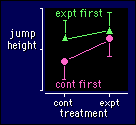
 The
figure shows data for an example of a simple crossover, in which an experimental
treatment increased jump height relative to a control treatment. I've separated
the data for the two groups (control treatment first, experimental treatment
first) to illustrate a practice effect, which adds to the difference between
experimental and control treatments for the group that had the control treatment
first, but reduces the difference for the other group. The data also illustrate
that randomization of athletes to the two groups resulted in one group (expt
first) being somewhat better jumpers overall.
The model has the same form as the model at the top of this page, but the time effect is now replaced with treat, which has two levels (cont and expt). The other main effect, group, now represents which group each subject was assigned to (contfirst, exptfirst). The interaction term treat*group has four levels (cont·contfirst, cont·exptfirst, expt·contfirst, and expt·exptfirst).
The difference between the two levels of the treatment effect (expt - cont) tells you the thing you're most interested in: how well the treatment worked relative to control. The difference between the two levels of the group effect (exptfirst - contfirst) tells you how different your two groups of subjects were, so it's a measure of how well you randomized your subjects to the two groups. The interaction gives you the size of the practice effect, and I'll leave you to figure out that the appropriate contrast is 0.5*(expt·contfirst - expt·exptfirst - cont·contfirst + cont·exptfirst ). If that's too challenging, here's another way to get the practice effect. First, make another repeated-measures variable called trial in your data set. Trial is almost the same as treat, but trial has values of the dependent variable corresponding to the first and second trial, whereas treat has values corresponding to control and experimental treatments. Now do the ANOVA with group, trial, and group*trial in the model. The practice effect comes straight from trial in this model.
Get your stats program to give you confidence intervals for all these contrasts, please, not just the p values! And if you plot your data for publication, show the two groups as I have done in the above example.
A bonus for this method of analyzing crossovers is no absolute
requirement for an equal number of subjects in each group. It's still
best to have equal numbers, but if you get dropouts in one group, the
resulting treatment effect is not biased by any practice effect. It
would be biased if you used a paired t test to analyze the data.
Users of the Statistical Analysis System have the option of modeling
the data in a slightly more intuitive way. Instead of having a group
effect in the model, use a variable called trial, which has values
first and second (or 1 and 2). This
variable indicates whether the given observation represents each
subject's first or second trial or test. Here's the model:
model: numeric <= (subject) treat trial treat*trial
It looks similar to the previous model, but trial is actually a second within-subject factor, which we haven't dealt with yet. It turns out that traditional methods of repeated-measures ANOVA can't handle this model, because each subject has values for only two of the four combinations of treat and trial. But the new mixed procedure in SAS handles it brilliantly. Just use the treat term to get the estimate of the difference between the experimental and control treatments, and use the trial term to get the practice effect. An appropriate combination of the levels of treat*trial gives the difference between the means of the two groups of subjects with treatment and practice effects partialed out, if you want to check how evenly the subjects were randomized to the two treatment sequences.
The above models can be generalized to
multiple crossovers:
crossovers with several treatments. More about those after the next
page, which deals with more than two trials.
Go to: Next · Previous · Contents · Search
· Home
editor
Last updated 8 Jun 2003